SQL Query Optimization: Understanding Key Principle
submited by
Style Pass
This guide is intended to help you gain a true understanding of SQL query speeds. It includes research that demonstrates the speed of slow and fast query types. If you work with SQL databases such as PostgreSQL, MySQL, SQLite, or others similar, this knowledge is a must.Working in a software development business gives a lot of understanding of the developer's skills. More and more, I have seen good YANG programmers who know their language and technology perfectly, follow trends, and take the time to learn about different approaches and libraries. Sometimes they even try to argue their "super-fast code" which in fact saves a couple of CPU loops but decreases readability. But when they start working with databases, these developers tend to produce very expensive queries that take an infinity when dealing with thousands or millions of records in the table. They often get stuck here, unable to address the problem and unsure what to even Google to get started. Sometimes such issues occur in SQL databases, other times in NoSQL. Though the basic principle of data access speed is common everywhere, and not so complex as it looks from first sight.No worries if it familiar to you, here I will explain one by one how to make your queries fast. I will write in the simplest way I can because my aim is that anyone with or without database knowledge can understand the principle which distinguishes slow and fast data handling. This principle in all situations where data access speed is important. If you spend half an hour reading this guide, you may very well use the knowledge you gain for years to come.Here are the three basic terms related to a data handling performance that I’ll explain, as simply as possible:Code complexity O(x)Binary treesIndexesUnderstanding the problem of slow application is a first what you need to doConsider a doctor who can make an educated guess about a patient's ailment just by looking at their face. Their judgment and viewpoint are shaped by years of experience. Some amount of real-world experience is a must for all of us. But here, I’ll try to help you avoid some trial-and-error time, so that you’ll be ahead of the pack, rather than scrambling to catch up.Every app is different, and bottlenecks are caused by different factors, but every programmer who is working with data knows that bottleneck in most cases comes from data storage. Both blocking and asynchronous programming implementations do rely on one centralized database, so even one slow query in the database makes a huge impact on whole application performance. Especially if it is an oftenly executed query.The truth is that each query could be classified into two kinds: Query which time grows with table rows countQuery which time is constantly small for any amount of rows in the tableThe first one is the worst case because it is hard to note during local development but with each piece of new data is becomes worsen and worsens, and then it turns into a big Snowball which makes your app irresponsible. Another sad thing that it is hard to note even in or production environment: most web apps never used with predictive smooth distribution (saying 1 user per minute). The users of most services getting inside by Erlang distribution law (most time they are sleeping, but during dinner, they all visit your site with memes, at the beginning of they all check email, at the afternoon they watch streams on your streaming platform). So when you as the site owner will check performance at random times during the day, it might fully crash on spikes of usage.If you already have performance issues, before starting turning kind 1 into kind 2 you need to find all query times for kind 1. To do you can use special database tooling. Every database has a slow query log that logs all queries which took more than xx ms. The threshold is easily configurable. If you face any performance issues on your data-based app, start with enabling a slow log.The idea is to prioritize fixing queries that make the most impact on performance. So you need to match which request makes a slow query, estimate how often it is, and then start optimizing it. What makes SQL queries in databases slow?To start, let's imagine a simple data table: Now, we will make a query to the database to check whether the user with the name Evan exists in the table. The database will check the lines, one by one, and compare the name field in the table with the target value. All data in most databases are stored on a hard drive. So the DB will read the item with ID 1, will fetch the field name, and will compare it with "Evan." "Adam" is not equal to "Evan", so the DB will go to the next line. And so on. So, in this particular example, the DB will take seven reads and make seven string comparisons.If we would run a query that checks whether the name "Luke" is in the table, there will be a total of eight operations. With a growth of a client base, though, a table like this might reach 10,000 users - that means up to 10,000 operations to check a name!Here we come to the term of Complexity.Complexity is defined as a function that describes how many operations you need to perform to get a result. It’s usually symbolized by O(x), where x is a function of N, where N is a total number of possible operations.In our case, we see a linear function – our maximum number of operations is N, where N is the number of items in the table. We can write this as O(N). This represents the complexity of a given DB query.How to make search fasterDid you use a vocabulary textbook in school? You had a book with three thousand pages but were able to find any given word pretty quickly. How did you do it?The answer is simple enough – all words in this book were sorted alphabetically. So, you opened a book in the middle and compared the first letter of your target word with the first letter of the words on the current page. You knew if your letter is earlier in the alphabet, you moved to ~ 1/4 of the way through the book. Then you repeated and moved another ~1/8 of the book forward or backward. So, it took several iterations to find a word, but the overall process was quick.This method is called Dichotomy or binary division. You may also hear it called the Phone Book principle. Old, non-digital phone books worked under the same principle -they sorted people’s or company’s names alphabetically(one of the original benefits to Apple’s company name was that it placed their listing towards the beginning of the phone book).Let's imagine we can resort our table: Now we need to find Evan. We select a middle item: 6 Jerry, and compare words: Evan is less than Jerry ( E < J), so we split the first 4 items by 2 and get 2 Bruce.Evan is greater than Bruce ( E > B ) so we go to the middle of the range and get Evan.Evan equal to Evan, so we found that the item existsThree operations instead of eight. Sounds better? You can create a larger table and calculate how many iterations it would take. In the end, you will find that the binary division method always gives O(log2(N)) complexity. I will show some simple DB research in the sections below, accompanied by charts so you can see how and why this is the case. The log2 function is the best complexity ever - that’s because a significant growth of the number of items yields only a very small growth of the function:Log2 (4) is 2Log2 (8) is 3Log2 (16) is 4Log2 (32) is 5 Log2 (1,024) is 1 0Log2 (2,048) is 11Log2 (10,000,000) is 24Log2 (100,000,000,000) is only 36Is that not awesome? We can have 100,000,000,000 items in the table and will need only 36 comparisons!If we plot O(N) and O(Log2(N)) on chart for N = 1..10, here’s what we get: However, for N = 1..500 the growth of Log function is hard to even notice, compared to linear function growth: Implementation of the phone book principle in computers and databasesGenerally, it would not take a lot of time for you to implement a phone book binary division search via a plain linear array. It will give you Log2 complexity, but each iteration would take mathematics to divide indexes. So computer scientists created another, more optimal data structure that works in the same way but does not require indexes arithmetics.This called Binary Tree or just BTree. And no need to fear, BTree is a very simple and smart idea!Let's consider how to turn our table into a binary tree: Next comes the search method:We always start searching from the root node. Evan < Jerry (E < J) so we need to move to the left daughter nodeNow we are on Bruce, and Evan > Bruce so we move towards the right daughter node.We got Evan equal to Evan. This method has the same O(Log2(N)) complexity. We just followed a tree from top to bottom: This time we did three comparisons and followed two arrows. If we needed to find a John, it would take four comparisons and three arrows. The longest possible path is three.You can create another example with 16 nodes in the tree and still ensure that the longest path (number of arrows) won’t exceed Log 2 (16) = 4.A binary tree, just by its natural look, shows perfectly the whole principle of the logarithm function. Here are 35 nodes on the tree, and the depth of the tree is equal to 5: Indeed Log2(35) is 5.129, or 5 if we round to integer.Inside of a DB, all table items can be linked to a binary tree. However, each table might need fast searches on different fields.For example, I might want to search IDs by Names, or Names by IDs. That's why we might have two different trees. In real databases, it is much more efficient to store not copies of whole nodes, but addresses to real nodes’ storage. Review the image above carefully to understand how it works. It is the closest example to a real database. As we can see, there are two indexes implemented with different binary trees. Each node points to a table item. A table item might be pretty heavy due to long VARCHAR/TEXT fields, but it’s nevertheless easy to address the item on disk because the Tree node will give us a direct pointer to the space on disk which holds a whole item with all its fields.Taking on this approach, we can debunk one big myth – some developers believe that every additional column makes queries slower, and so try to minimize the number of columns. If you understood the principle above, you will never make such fooling assumptions. Yes, additional columns will take up more space on a hard drive. Yes, they might consume more network traffic in the channel between your app and DB server (but you could just store some columns without transferring them over connection every time).Obviously, trees for the index should be formed during INSERT queries. Inserting is also very fast - we should just find a place to insert to keep out less than/more than logic which is O(Log2(N)) and then put time and pointer. However, if a lot of several inserts will come into the same branch, the tree will become less efficient, so there is a special rotating mechanism to keep order but reduce depth. This is a simple process but I will not dig so deeply now.Let's make real research to prove itLet's put our table into practice and measure the time of SELECT for a different number of elements.To simplify experiments, you’ll need some programming language apart from pure SQL. My choice is NodeJS without ORM, because most of us know JavaScript today.As a database, I will use Postgres v12, though you can use any SQL DB - the syntax will be plus/minus the same.If you don't know how to get PostgreSQL and create a superuser, please follow the install and setup PostgreSQL guide. Login to psql CLI:su -c psql postgres Create database and user:CREATE DATABASE testdb ENCODING 'utf-8' ; CREATE USER researcher with LOGIN SUPERUSER ENCRYPTED password 'passw1' ;To exit psql CLI, type Ctrl+DI created a public GitHub repo - devforth/sql-query-benchmark - which makes all the experiments I want to show. Code connects to the database, creates a table with index, and starts to make inserts. For every 4,000 inserts, SELECT time is measured. To visualize the results, the code runs a simple web server that serves pages with charts. It also has a WebSocket connection to update data as soon as possible.To run the code, we need Node v12 or later.Here’s how to install it:git clone https://gi thub.com/devforth/ sql-query-benchmark.git npm ciAnd here’s how to run an experiment:node index .jsSearching on a name column that has no indexThe code of the first experiment does next: seeder = randomSeed.create (RAND_SEED); await pool.query(`CREATE TABLE ${TABLE_NAME } ( id serial PRIMARY KEY , name VARCHAR (50 ) );`,); // word against we will search , let it make 100 % non existing to make sure we are at the worst case search_word = gen_unique_string(NAME_FIELD_VALUE_LENGTH); await runexp( 'Select by "name" without Index on "name"' , { text : `INSERT INTO ${TABLE_NAME } (name ) VALUES ($1 );`, dataGenerator: (i) => [gen_random_string(NAME_FIELD_VALUE_LENGTH, seeder)], }, { text : `SELECT FROM ${TABLE_NAME } WHERE name = $1 ;`, dataGenerator: (i) => [search_word], } );Seeder is a random generator with a fixed seed. Fixed seed guarantees that the sequence of random numbers will be the same from one experiment to another. So, generated data for each experiment will be the same.The search_word is a word with a length of 10 characters, which 100% will not be generated with seeder. So, we will select this word, and it will never be found. That gives us the worst-case scenario.The runexp is a function that makes an experiment and measurements. The first parameter is a name used for chart and CSV filename with actual timing (the source data of the chart). The second parameter is an INSERT query and data for each iteration. The third parameter is a SELECT code.How it works:The script inserts a row, one by one, using an INSERT query. From 1 to 100,000.Every 4k INSERTs script runs a series of SELECTs to measure select time gains for our unique word as well as the current count of inserted rows in the table. We repeat SELECT 3k times to find a better smooth average. Single’s select time might vary because of CPU usage, spikes, or database server payload entropy.With SELECT, for every 4k records, we also calculate an INSERT average time. What if it is also changed?Here is what I got: Select time on 4k rows: 0.265 ms, on 100k rows: 5.652 ms. So with every 10k items, time increases by ~0.56ms. This is exactly how O(N) should look. For one million rows, we should get 56 ms, for one hundred million, we should get 5.6 seconds.Insert time looks like a constant. On 4k rows, one insert time is 0.017 ms, on the last, it is 0.015 ms.Now let's create an index on the name field: await pool.query(`CREATE INDEX index1 ON names (name );`);Here’s the full code of the experiment: seeder = randomSeed.create (RAND_SEED); search_word = gen_unique_string(NAME_FIELD_VALUE_LENGTH); // cleanup all table before new experiment await pool.query(`DROP TABLE ${TABLE_NAME };`); await pool.query(`CREATE TABLE ${TABLE_NAME } ( id serial PRIMARY KEY , name VARCHAR (50 ) );`,); await pool.query(`CREATE INDEX index1 ON ${TABLE_NAME } (name );`); await runexp( 'Select by "name" with index on "name"' , { text : `INSERT INTO ${TABLE_NAME } (name ) VALUES ($1 );`, dataGenerator: (i) => [gen_random_string(NAME_FIELD_VALUE_LENGTH, seeder)], }, { text : `SELECT FROM ${TABLE_NAME } WHERE name = $1 ;`, dataGenerator: (i) => [search_word], } );Result: As you can see, select time now looks like a constant line near 0.02 ms for one SELECT query, which is even faster than one INSERT. In the end, there is a small fall down to 0.012 ms which could be related to the "Smartness" of the Postgres query planner or tree rotator. But this is not significant, and it probably occurred on the previous chart as well. Actually, the bottom line is not constant but is instead based on O(Log2(N)). It will grow but only very slowly, as we have shown before. You can think about it as essentially being a constantly low value.On 100k, we improved speed by 466 times! On one million, we would improve time by 4666 times.Select time: this is exactly how O(N) looks in real life. Each 5k inserts make a request slower by ~0.3msInsert time: almost constant with minor fluctuations from 0.03 up to 0.04ms☝ Conclusion: always create indexes for the field which you use in your SELECT WHERE statement. By the way indexes for all PRIMARY KEY types as IDs are created by the Database already.Searching on multiple fields' speeds: composite indexLet's add the third field (integer age) and try to SELECT on both fields: seeder = randomSeed.create (RAND_SEED); search_word = gen_random_string(SHORT_NAME_FIELD_LENGTH, seeder); await pool.query(`DROP TABLE ${TABLE_NAME };`); await pool.query(`CREATE TABLE ${TABLE_NAME } ( id serial PRIMARY KEY , name VARCHAR (50 ), age INTEGER );`); await pool.query(`CREATE INDEX index1 ON ${TABLE_NAME } (name );`); await runexp( 'Search on "name", "age" with index on "name" only' , { text : `INSERT INTO ${TABLE_NAME } (name , age) VALUES ($1 , $2 );`, dataGenerator: (i) => [gen_random_string(SHORT_NAME_FIELD_LENGTH, seeder), 10 + seeder(100 ) ], }, { text : `SELECT FROM ${TABLE_NAME } WHERE name = $1 and age = $2 ;`, dataGenerator: (i) => [search_word, 1 ], } );To show the true consequences of the experiment, I forced the conditions to make sure there will be a lot of matching names. To achieve this, instead of generating a unique string, we generate a random string of the length 1. Our alphabet is only 2 chars - A and B - so ~50% of rows will be matched by the names column. Here we unleash the next level search for age (if we were to have only one name or not have found a name at all, there would be nothing for the DB to do). Yes, this is O(N) once again. But you’ll find that, interestingly, this experiment is a little bit faster than the first experiment (1ms faster on 100k). Why? Because we have an old index on "name," and it helps to find clusters with name matching items faster. Then it again has to try all items in the cluster to find age.To fix it, we need to create a so-called composite index on two columns, which looks like this:CREATE INDEX index1 ON names (name , age);It is the same binary tree, but instead of one value you can think about it as a combination of values, like AB:37. This makes it so easy to find a combination of two values by following ordered pairs.Here’s the whole code: seeder = randomSeed.create (RAND_SEED); search_word = gen_random_string(SHORT_NAME_FIELD_LENGTH, seeder); await pool.query(`DROP TABLE ${TABLE_NAME };`); await pool.query(`CREATE TABLE ${TABLE_NAME } ( id serial PRIMARY KEY , name VARCHAR (50 ), age INTEGER );`); await pool.query(`CREATE INDEX index1 ON ${TABLE_NAME } (name , age);`); await runexp( 'Search on "name", "age" with index on "name", "age"' , { text : `INSERT INTO ${TABLE_NAME } (name , age) VALUES ($1 , $2 );`, dataGenerator: (i) => [gen_random_string(SHORT_NAME_FIELD_LENGTH, seeder), 10 + seeder(100 ) ], }, { text : `SELECT FROM ${TABLE_NAME } WHERE name = $1 and age = $2 ;`, dataGenerator: (i) => [search_word, 1 ], } );And here’s the result: As we see that SELECT is fast again!☝ Conclusion: when you search by multiple columns, create a composite index that covers all of them.Reusing one index for several searchesReal web apps often need to make SELECTs in one table with different sets of fields. It might happen that one endpoint of your REST API searches by name + age, and the other by name only.So you might ask: Can I use my name + age index to search quickly by name as well?Well, let's see:seeder = randomSeed.create (RAND_SEED); search_word = gen_unique_string(NAME_FIELD_VALUE_LENGTH); await pool.query(`DROP TABLE ${TABLE_NAME };`); await pool.query(`CREATE TABLE ${TABLE_NAME } ( id serial PRIMARY KEY , name VARCHAR (50 ), age INTEGER );`,); await pool.query(`CREATE INDEX index1 ON ${TABLE_NAME } (name , age);`,); await runexp( 'Search on "name" with index on "name", "age"' , { text : `INSERT INTO ${TABLE_NAME } (name , age) VALUES ($1 , $2 );`, dataGenerator: (i) => [gen_random_string(NAME_FIELD_VALUE_LENGTH, seeder), 10 + seeder(100 ) ], }, { text : `SELECT FROM ${TABLE_NAME } WHERE name = $1 ;`, dataGenerator: (i) => [search_word], } ); As you see it works. Indeed a composite index would allow finding a pair of values Name + Age, but we are searching but the name is first in pair, so we can stop on it.However, there is a very important notice: order of fields in index matters: currently we had index on name+age and searched by name. Let's see whether it works if we will have an index on age+name and search by name: seeder = randomSeed.create (RAND_SEED); search_word = gen_unique_string(NAME_FIELD_VALUE_LENGTH); await pool.query(`DROP TABLE ${TABLE_NAME };`); await pool.query(`CREATE TABLE ${TABLE_NAME } ( id serial PRIMARY KEY , name VARCHAR (50 ), age INTEGER );`,); await pool.query(`CREATE INDEX index1 ON ${TABLE_NAME } (age, name );`,); await runexp( 'Search on "name" with index on "age", "name"' , { text : `INSERT INTO ${TABLE_NAME } (name , age) VALUES ($1 , $2 );`, dataGenerator: (i) => [gen_random_string(NAME_FIELD_VALUE_LENGTH, seeder), 10 + seeder(100 ) ], }, { text : `SELECT FROM ${TABLE_NAME } WHERE name = $1 ;`, dataGenerator: (i) => [search_word], } );And... It did not work, because pairs of values in the tree now begin with age: 33:BA . So the tree is not sorted by name anymore.What to do in such cases? Remember that you can create multiple indexes. In our case we will create one on age + name and another on name only:seeder = randomSeed.create (RAND_SEED); search_word = gen_unique_string(NAME_FIELD_VALUE_LENGTH); await pool.query(`DROP TABLE ${TABLE_NAME };`); await pool.query(`CREATE TABLE ${TABLE_NAME } ( id serial PRIMARY KEY , name VARCHAR (50 ), age INTEGER );`,); await pool.query(`CREATE INDEX index1 ON ${TABLE_NAME } (age, name );`,); await pool.query(`CREATE INDEX index2 ON ${TABLE_NAME } (name );`,); await runexp( 'Search on "name" with index on "age", "name" + index on "name"' , { text : `INSERT INTO ${TABLE_NAME } (name , age) VALUES ($1 , $2 );`, dataGenerator: (i) => [gen_random_string(NAME_FIELD_VALUE_LENGTH, seeder), 10 + seeder(100 ) ], }, { text : `SELECT FROM ${TABLE_NAME } WHERE name = $1 ;`, dataGenerator: (i) => [search_word], } );And: It is fast again!☝ Conclusion: to simplify things, prevent human errors and improve code readability, always create one index for one unique SELECT query. If one select compares 4 fields and another 2 fields, then create 1 index for 4 fields and another for 2 fields.How to speed up ORDER BYSome of your queries might need to select items ordered by some field. In our case, if we assume we store humans, it might be – "Find oldest John". We know there are a lot of Johnes. Again let's increase the probability of the same name and try it with only one index on the name:seeder = randomSeed.create (RAND_SEED); await pool.query(`DROP TABLE ${TABLE_NAME };`); await pool.query(`CREATE TABLE ${TABLE_NAME } ( id serial PRIMARY KEY , name VARCHAR (50 ), age INTEGER );`); await pool.query(`CREATE INDEX index1 ON ${TABLE_NAME } (name );`); search_word = gen_random_string(SHORT_NAME_FIELD_LENGTH, seeder); await runexp( 'Search top 1 with exact "name" ordered by "age" (oldest) descending with index on "name" only' , { text : `INSERT INTO ${TABLE_NAME } (name , age) VALUES ($1 , $2 );`, dataGenerator: (i) => [gen_random_string(SHORT_NAME_FIELD_LENGTH, seeder), 10 + seeder(100 ) ], }, { text : `SELECT FROM ${TABLE_NAME } WHERE name = $1 ORDER BY age DESC LIMIT 1 ;`, dataGenerator: (i) => [search_word], } ); Not the best performance. What we need is to field age with desc specifier as another field to the index.CREATE INDEX index1 ON names (name , age desc );The order of fields in the index always matters! First, we specify fields which used in WHERE, then fields used in ORDER BY. If several fields are used in ORDER BY, you need to follow the same order as used in select.Full code: seeder = randomSeed.create (RAND_SEED); search_word = gen_random_string(SHORT_NAME_FIELD_LENGTH, seeder); await pool.query(`DROP TABLE ${TABLE_NAME };`); await pool.query(`CREATE TABLE ${TABLE_NAME } ( id serial PRIMARY KEY , name VARCHAR (50 ), age INTEGER );`); await pool.query(`CREATE INDEX index1 ON ${TABLE_NAME } (name , age desc );`); await runexp( 'Search top 1 with exact "name" ordered by "age" descending (oldest) with index on "name", "age desc"' , { text : `INSERT INTO ${TABLE_NAME } (name , age) VALUES ($1 , $2 );`, dataGenerator: (i) => [gen_random_string(SHORT_NAME_FIELD_LENGTH, seeder), seeder(100 ) ], }, { text : `SELECT FROM ${TABLE_NAME } WHERE name = $1 ORDER BY age desc LIMIT 1 ;`, dataGenerator: (i) => [search_word], } );Good speed again: Yes, we see some very minor fluctuations here, but the lowest value is 0.02 ms still which Is extra small comparing to the previous experiment result, and the trend line would be based on log2(N) anyway.Searching multiple items after ORDER BYHere is one challenging moment. If we try to get a full cluster of ordered elements, we will see worsen results: seeder = randomSeed.create (RAND_SEED); search_word = gen_random_string(SHORT_NAME_FIELD_LENGTH, seeder); await pool.query(`DROP TABLE ${TABLE_NAME };`); await pool.query(`CREATE TABLE ${TABLE_NAME } ( id serial PRIMARY KEY , name VARCHAR (50 ), age INTEGER );`); await pool.query(`CREATE INDEX index1 ON ${TABLE_NAME } (name , age desc );`); await runexp( 'Search all with exact "name" ordered by "age" descending with index on "name", "age desc"' , { text : `INSERT INTO ${TABLE_NAME } (name , age) VALUES ($1 , $2 );`, dataGenerator: (i) => [gen_random_string(SHORT_NAME_FIELD_LENGTH, seeder), seeder(100 ) ], }, { text : `SELECT FROM ${TABLE_NAME } WHERE name = $1 ORDER BY age desc ;`, dataGenerator: (i) => [search_word], } ); Do you remember that each index stores pointers to elements? Though results are stored in Tree, the Database server needs to resolve pointers for each element to return it in sequence. So the index might work even worse as states Postgress documentation about indexes for ORDER BY.However, this case is pretty rare because most systems for large output data use paginations with a page for 10 - 20 elements, so the index will work: in our example, we tried to resolve ~ half of a table with links, which is ~50k at 100k point. But database would quickly resolve 10 - 100 elements.☝ Conclusion: if your query has ORDER BY then your index containing only where the field will not work for it. Always pay attention to ordering and include the fields of ORDER BY in the indexDoes order direction matters for index (acceding/descending)In the previous example, we sorted using DESC direction and specified DESC in the index also. Let's leave the index the same but try to use another direction for query: seeder = randomSeed.create (RAND_SEED); search_word = gen_random_string(SHORT_NAME_FIELD_LENGTH, seeder); await pool.query(`DROP TABLE ${TABLE_NAME };`); await pool.query(`CREATE TABLE ${TABLE_NAME } ( id serial PRIMARY KEY , name VARCHAR (50 ), age INTEGER );`); await pool.query(`CREATE INDEX index1 ON ${TABLE_NAME } (name , age desc );`); await runexp( 'Search top 1 with exact "name" ordered by "age" ascending (youngest) with index on "name", "age desc"' , { text : `INSERT INTO ${TABLE_NAME } (name , age) VALUES ($1 , $2 );`, dataGenerator: (i) => [gen_random_string(SHORT_NAME_FIELD_LENGTH, seeder), seeder(100 )], }, { text : `SELECT FROM ${TABLE_NAME } WHERE name = $1 ORDER BY age asc LIMIT 1 ;`, dataGenerator: (i) => [search_word], } );And: Looks pretty good. So items were sorted by age and it still quickly found items on the other end of each name cluster.But I would not recommend you doing it if you are ordering on multiple fields. Here game changes dramatically. Let's add the deposit field. Nowe index includes 3 fields. CREATE INDEX index1 ON names (name , age desc , deposit desc );But let's order on:ORDER BY age asc , deposit desc LIMIT 1 The experiment code: seeder = randomSeed.create (RAND_SEED); search_word = gen_random_string(SHORT_NAME_FIELD_LENGTH, seeder); await pool.query(`DROP TABLE ${TABLE_NAME };`); await pool.query(`CREATE TABLE ${TABLE_NAME } ( id serial PRIMARY KEY , name VARCHAR (50 ), age INTEGER , deposit INTEGER );`); await pool.query(`CREATE INDEX index1 ON ${TABLE_NAME } (name , age desc , deposit desc );`); await runexp( 'Search on "name" items ordered by "age" ascending, "deposit", descending with index on "name", "age desc", "deposit desc" ' , { text : `INSERT INTO ${TABLE_NAME } (name , age, deposit) VALUES ($1 , $2 , $3 );`, dataGenerator: (i) => [gen_random_string(SHORT_NAME_FIELD_LENGTH, seeder), seeder(100 ), seeder(200 )], }, { text : `SELECT FROM ${TABLE_NAME } WHERE name = $1 ORDER BY age asc , deposit desc LIMIT 1 ;`, dataGenerator: (i) => [search_word], } );As you can see we lost ~0.2 milliseconds on 100k elements so it would obviously continue to increase. To fix it, always sync ordering in real query with index: seeder = randomSeed.create (RAND_SEED); search_word = gen_random_string(SHORT_NAME_FIELD_LENGTH, seeder); await pool.query(`DROP TABLE ${TABLE_NAME };`); await pool.query(`CREATE TABLE ${TABLE_NAME } ( id serial PRIMARY KEY , name VARCHAR (50 ), age INTEGER , deposit INTEGER );`); await pool.query(`CREATE INDEX index1 ON ${TABLE_NAME } (name , age, deposit desc );`); await runexp( 'Search top 1 with exact "name" ordered by "age" ascending, "deposit", descending with index on "name", "age asc", "deposit desc" ' , { text : `INSERT INTO ${TABLE_NAME } (name , age, deposit) VALUES ($1 , $2 , $3 );`, dataGenerator: (i) => [gen_random_string(SHORT_NAME_FIELD_LENGTH, seeder), seeder(100 ), seeder(200 )], }, { text : `SELECT FROM ${TABLE_NAME } WHERE name = $1 ORDER BY age asc , deposit desc LIMIT 1 ;`, dataGenerator: (i) => [search_word], } );Good again: ☝Conclusion: to simplify things, prevent human errors, and improve code readability, always create one index for different directions in order by. If you have one SELECT ordering a asc, b desc, and another doing a asc, b ask, create two indexes.This should be enough to activate your brain when your writing queries. I would recommend to re-check all results carefully several times, finding all differences in a code. Also now you have a repo which you can fork and perform any experiment which would come to your mind.Unique and non-unique indexesIn the example we created indexes using:CREATE INDEX index0 ON t (a, b);This means there might exist two pairs with the same a value and b value combination. This would be not possible if we do:CREATE UNIQUE INDEX index0 ON t (a, b);And this is the main difference. If you think unique indexes would give a better performance – try it by yourself.Some indexes already created for youLogin to psql CLI, then connect to db:\connect testdb; And create a table:CREATE TABLE example ( id serial PRIMARY KEY , name VARCHAR (50 ) );Now let's check out the created table information:\d+ example Binary Tree index already created for ID column. Why? It happened because we marked the field as PRIMARY KEY. Al PKs have indexes because they are widely searched.The endI believe that managing data skills in a fast and "cheap payload" way is a key to the success of the most modern software. Hope you enjoyed important knowledge you received from me.Contact me by comments if you have any further questions or want to learn about other optimization best practices, for example how to not use slow JOINS and apply data denormalization to achieve maximum speed. Related links:MySQL Indexes and PerformancePostgreSQL IndexesPostgreSQL Indexes and ORDER BYSQLite Indexes
This guide is intended to help you gain a true understanding of SQL query speeds. It includes research that demonstrates the speed of slow and fast query types. If you work with SQL databases such as PostgreSQL, MySQL, SQLite, or others similar, this knowledge is a must.
Read more hinty.io/dev...
Leave a Comment
Related Posts


Recent Posts


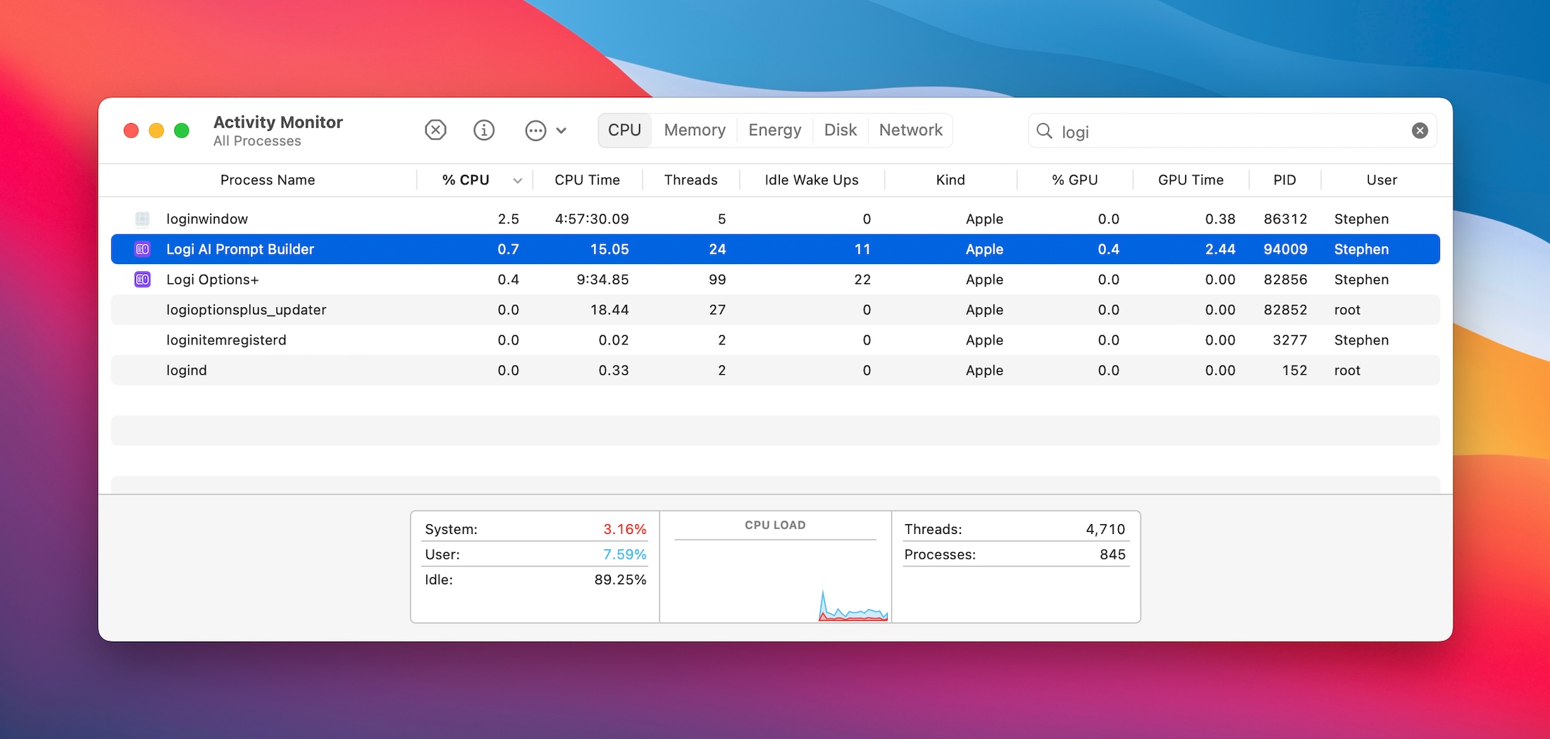
Logitech’s Mouse Software Now Includes ChatGPT Support, Adds Janky ‘ai_overlay_tmp’ Directory to Users’ Home Folders
Comment

/cloudfront-us-east-1.images.arcpublishing.com/pmn/2OMDYOYIKRDYJOSDNJCST4GN34.jpg)